I got the idea from a YouTube video. Someone was demoing a temporary email service: open the page, get an address, wait for your verification code. It worked fine, but the whole thing was one tab you had to babysit. I figured I could do better.
The obvious improvement: stop making you come to the inbox. Put it in the browser toolbar. Have it fill in signup forms. Ping you when mail arrives. And while I was at it, fix the part where every temp-mail service keeps a copy of everyone’s mail on its servers.
So that’s what sveltemail is: a dead drop with end-to-end encryption. Your browser makes its own key when it mints an inbox, and the private half never leaves your machine. What sits on our servers is ciphertext: steal our database tomorrow and you’d walk away with noise. The second your browser gets a message, we delete our copy too.
Try it right here
Live demo: this is the real sveltemail inbox, running right inside this post. Mint an address and watch it work.
Take it with you: the Firefox extension
If you’d rather have the inbox in your toolbar than in a tab, there’s a Firefox extension now. It mints a fresh address for every form you fill, autofills it in one click, and lets you know when new mail lands.
No accounts, ever. Your address is a random token with nothing attached to it: there’s nothing to leak.
Tracking pixels die at the door. HTML mail gets sanitized before you see it: remote images, scripts, all the exfiltration tricks, stripped out.
Inboxes live 5 to 30 minutes: your pick. Timer hits zero: it’s gone.
What I really want is for this to be easy to reach however you work. The Firefox extension is out now: one-click addresses, form autofill, new-mail notifications right in the toolbar. Chrome and Safari are next.
Last night, I spent several hours conversing with Perplexity AI in this session to understand various quantum phenomena better, including the math and general concepts behind: Quantum Tunneling, Quantum Annealing, and Quantum Energy Teleportation.
As a result of my work, I then took it to Gemini Deep Research to have it organize everything better than my sporadic, adhoc style of research had been. The result of that work is available on this site by clicking the image above.
The hope is that you can start with this research and start your own journey towards understanding quantum mechanics and how they can be used to break down geometrically complex problem spaces that cannot be solved by classical means into much smaller problem spaces that can be solved in reasonable amounts of time.
In the last portion of our three-part series, we will be reviewing some of the code behind the Simple Moving Average (SMA) and Exponential Moving Average (EMA) predictive indicators that we have developed. Specifically, we will spend a little bit of time looking at the EMA Projection and the EMA Projection Trend indicators, since these have seemed to be the most useful ones thus far.
Before we get into it, I would like to introduce you to the Huddle, a place where we can crowd around, look at quantitative analytics code, and share ideas. Think of it as a community of ideas and concrete code in a format that is a bit less formal than a traditional code repository might be.
EMA Projection
First up, we have the EMA Projection, which is just our standard EMA plus a projection of where it should land at the current T0. It can make that projection two ways. The first, AverageSlope, takes the gross slope of our line as
m = dx / dy
dx = EMA_at_T_minus_1 - EMA_at_T_minus_period_minus_1
dy = Period  # T-1 back to T-(Period+1) spans
             # exactly Period bars
The second, PriceHold, is the default. It asks a simpler question: where would the EMA land if this bar closed exactly where the last one did? Thanks to how the EMA is built, that works out to the last bar’s slope, scaled down a little:
k = 2 / (Period + 1)  # the EMA's own weight
m = (1 - k) * (EMA_at_T_minus_1 - EMA_at_T_minus_2)
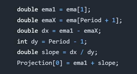
Specifically, the code that matters looks more like this in the real deal:
int lookback = ProjectionMethod == EMAProjectionMethod.AverageSlope ? Period + 1 : 2;
if (CurrentBar < lookback) {
	return;
}

double ema1 = ema[1];
double slope;
if (ProjectionMethod == EMAProjectionMethod.AverageSlope) {
	// ema[1] back to ema[Period + 1] spans Period bars.
	double emaX = ema[Period + 1];
	slope = (ema1 - emaX) / Period;
} else {
	// PriceHold: if this bar closes where the last one did, the EMA moves by
	// k * (Input[1] - ema1), which by the EMA's recursion is (1 - k) * (ema1 - ema2).
	double k = 2.0 / (1 + Period);
	double ema2 = ema[2];
	slope = (1 - k) * (ema1 - ema2);
}
Projection[0] = ema1 + slope;
Specifically, ema is an EMA object that calculates our exponential moving average for us already. We do not have to perform all of that work again.
Period is a property that is passed into the object at runtime, and Projection is a time-series plot added to the object at runtime. By default, Period is 14.
As you can see, there’s nothing complicated about this code. The entire algorithm is really only a couple lines if you were to “golf” that code, but let’s leave it as it is for readability.
The AverageSlope method calculates the gross slope of the line over the last Period bars. We backtested it on ES futures and SPY against faster estimates, and that average lags: it pointed the wrong way on roughly 30% of bars and took a median of three to four bars to follow a turn. PriceHold had about half its error, which is why it is now the default. AverageSlope is still there if you want to compare the two.
EMA Projection Trend
Building on the code from the EMA Projection, we have the EMA Projection Trend. It is a simple extension to the EMA Projection, but it provides a much clearer view of momentum. Specifically, it shows the changes in the slope of our EMA Projection as a proxy of momentum, which is a proxy of volatility, where larger bars indicate more change in the trend.
Altogether, this indicator seems to respond well to trend changes and can let us catch rides after it confirms other leading indicators. At least I have enjoyed using it.
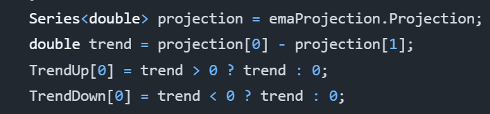
Without further delay, here is the entire algorithm:
As one can tell, it uses our EMA Projection. It performs a simple comparison of the T0 projection to the most recent prior projection at T-1. This shows us the trend and lets us see the momentum of our projection as it progresses.
The reason for TrendUp and TrendDown calculations being separate is because they are actually two different time-series plots. This allows us to choose distinct colors and is how we can show both green and red bars efficiently.
That’s All!
And with that, that’s all we have for today. This series is really supposed to be a three-part series, but having written what I have, I believe there is the possibility of some more talk on using moving averages as leading indicators.
Update, November 2026: we published a fix to the EMA Projection indicator. Its slope divided the change over Period bars by Period - 1, overstating it, and a backtest showed that averaged slope lagging, so the projection now defaults to PriceHold. The code above is the corrected version; see the fix on GitHub for the original and the backtest.
In the first part of our story, we discussed the Simple Moving Average (SMA) Projection line that showcased the SMA and a projection of the SMA in the next time step. From this, we could determine a little bit about volatility and also where the projections look like the current price action should be going.
I concluded my analysis of the SMA Projection as saying that I would not rely on it, but I think that I had spoken too soon. I performed more research on the idea and came up with another concept called the SMA Projection Trend, which is the same data, except it is instead represented as the difference between the current T0 projection and the most recent T-1 projection.
However, this will not be about the SMA Projection and SMA Projection Trend indicators. Instead, I have found more utility in the EMA Projection and Exponential Moving Average (EMA) Projection Trend indicators. The EMA is more responsive to immediate events and exponentially decays the more historic data to give a an average that is more biased towards recent data, which is important for traders that care about current price action.
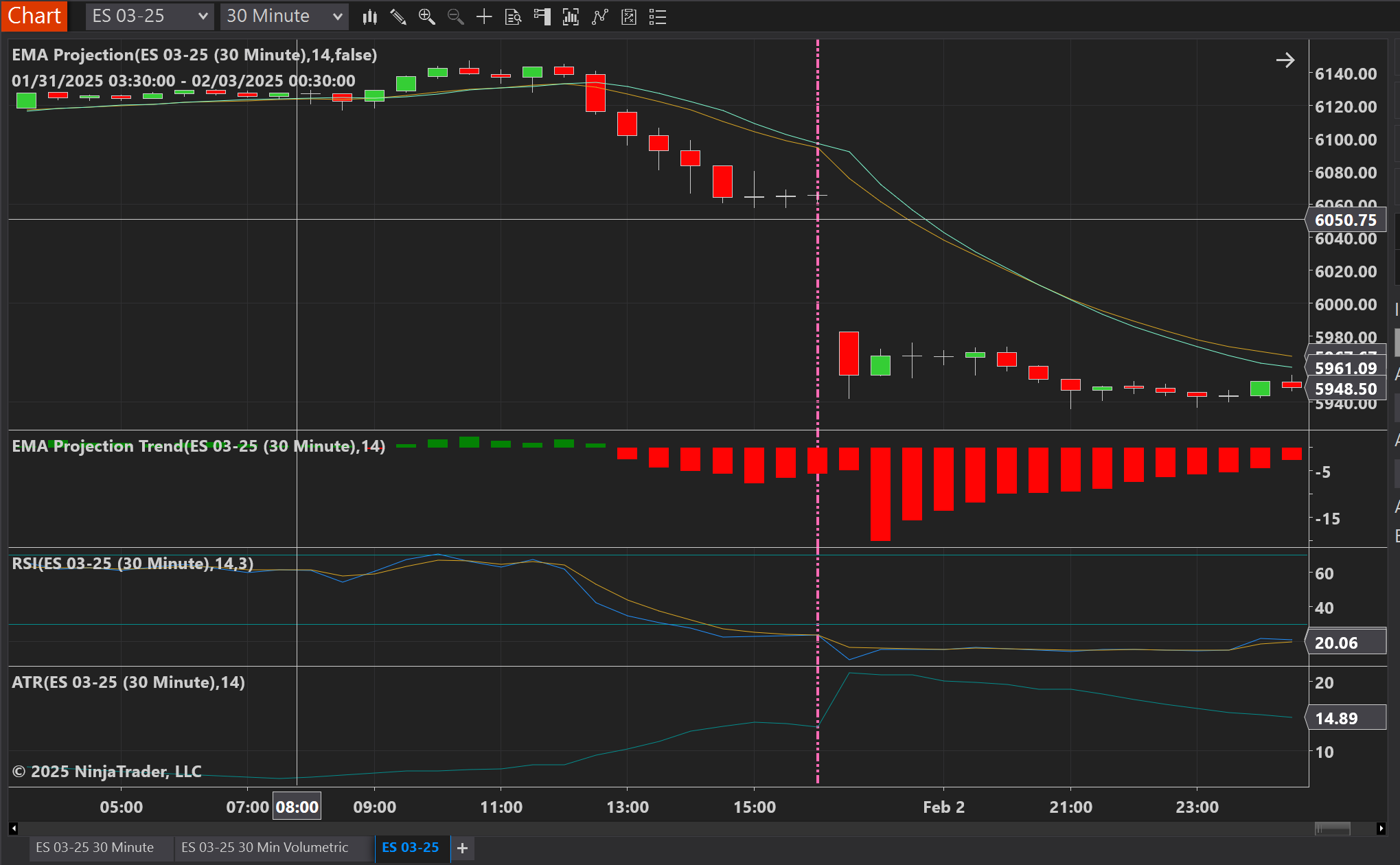
Whether talking about the SMA or EMA Projection Trends, they both measure momentum, which also takes into account volatility. For example, looking at the next chart, you can see captured momentum soon after the RSI crossed into overbought territory.
ES 30 minute chart with the EMA Projection overlaying the live data and the EMA Projection Trend displaying momentum in the graph beneath that.
To get a clearer picture, I have zoomed into the area of interest. For a 30 minute period, the RSI crossed into overbought territory before returning to normal. That was our first signal that we should begin paying attention for a good entrance, but we did not receive confirmation until three hours later that momentum was finally beginning to move downward.
Patience is key. The more confirmation signals you have, the more reliable your entrance.
RSI became overbought, and a few hours later, we receive our first indication that momentum is beginning to move in the expected downward direction.
In my opinion, we would have actually entered a short position three and a half hours after the RSI overbought signal, because we would have wanted to confirm that the close of the first downward momentum bar we saw actually closed down. Remember, patience is key, and before entering any position based on technical or fundamental data, acquiring a lot of confirming signals adds fuel to the fire for your entrance.
This is the time I would have recommended entering. It is right after we close on the first downtrend momentum bar after we had earlier seen the overbought signal on the RSI.
Use a critical eye. Nothing is guaranteed.
Combined with some other indicators, such as the ATR, RSI and perhaps the Bollinger bands if it suits you, the Projection Trend seems to be a pretty reliable detector. As a word of caution, however, you must look at the charts and these indicators with a critical eye, because unforeseen events can occur that lead them to lie to you. Therefore, always ensure you are paying attention to as much general information as you can.
To aid in preventing these pitfalls of unforeseen challenges, I recommend setting appropriate trailing stops. You can choose these to suit your own risk levels, but I would think the ATR can help you do this by looking at the total level of volatility over the last several bars of information. Perhaps you would want to do 2x ATR, or perhaps you would want to calculate the volatility through the Black-Scholes equation and use that to determine potential price movements. However you do it is an exercise left to the reader, but these are just some ideas.
Come back again as one more part to this series will be released that links to Happiness Enterprises’ github repo with these models in it. If you have Ninja Trader 8, you will be able to use them directly, and if not, well, you can at least translate the code to your own platform of choice.
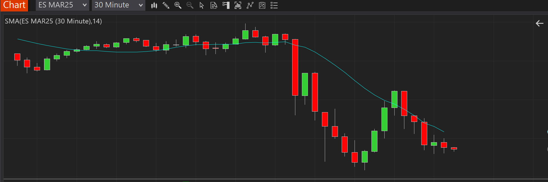
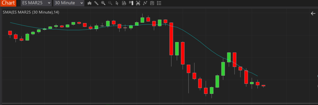
Everyone is likely familiar with the simple moving average (SMA). In trading, it is a lagging indicator used to visualize the average trend of price action over windows of time. Below is a chart with the SMA(14) plotted on it. Each data point corresponds with the average closing price of the 14 closing prices preceding it.
As you can see, the SMA(14) follows the general trend of the chart, but one thing is clear: it’s always lagging behind the actual price movement:
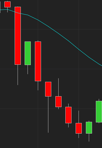
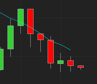
Visually, it appears that the SMA is shifted right of the price bars. In essence, they are, because the SMA lags. Also, since the SMA is an average of the previous prices, the curve is smoother and seems to travel somewhere close to the middle of the price action. Averages being averages, however, this will not always be the case.
So what can we do?
If moving averages are lagging, is there any way we can use them to predict the next value? Actually, there is.
Going back to geometry class, one might remember computing the slope of a line: y = dy / dx. The concept is simple enough: compute the difference in the average from the T-1 time to the T-(Tx+1) time. In our case, since we are assuming 14 time periods, then it would be T-15. The difference in time would then be 14, because there are 14 time periods separating time period T-1 from time period T-15.
Analysis
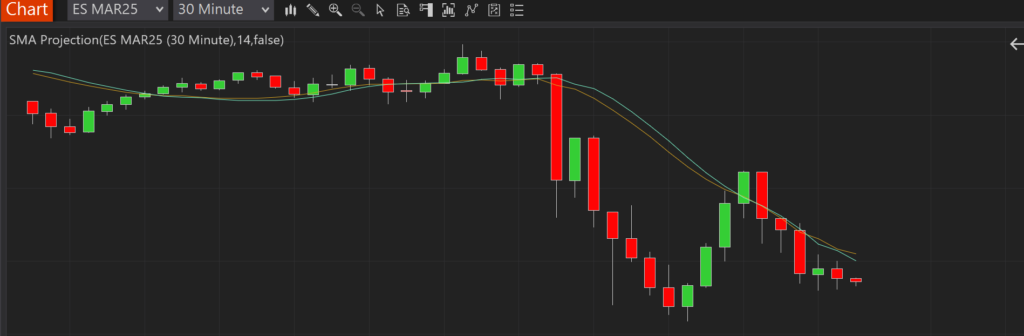
Given the above formula, let’s look at something we shall call the “SMA Projection”, because it can be used to project or predict the next value in the series based on the calculation of average price changes over time.
The color scheme above is a little different than earlier. This time, the goldenrod color is the SMA(14), and the aqua color is our SMA(14) projection.
Following the SMA(14) with the projection, we can consider a couple questions:
How far away from our projections were we compared to the SMA that was ultimately calculated? The closer we are, the less volatility there is, and the more accurately we have predicted where the average is moving.
How far away from our projections were we compared to the actual closing price? Again, the closer we are, the less volatility there is, and the more accurately we have predicted where price action is moving.
Can we trade based on this?
Looking closely at the above charts, it is possible to surmise some patterns that could lead to profitable trades:
If the open is below the prediction but the slope of the prediction is increasing, we could assume that price action is beginning to move upward in the direction of the averages, and we should enter long.
Conversely, if the open is above the prediction but the slope of the prediction is decreasing, we could assume that price action is beginning to move downward in the direction of the averages, and we should enter short.
Looking at the charts, we can see several possible opportunities like this. We can also see that there are several false positives as well.
Do we use this?
Personally, I would not use this as a very effective predictive measure on its own. Combined with Bollinger bands, it may be more effective, but it is still based on lagging data. The lag can be improved by shortening the time period of the SMA, but then it becomes more like looking at current price action rather than trends. If you want to play with that, however, you can try several, maybe starting with a period length of 5 rather than 14.
Conclusion
The point of this article was to serve as an easy-to-understand introduction to predictive analytics. Most people understand moving averages, and the simple moving average is the easiest of them all to grasp.
So what exactly is happening, and how can we leverage it? Well, predictive analytics basically involves determining the slope of a “line” or some other higher-dimensional surface and then predicting the next value on that surface by following the slope. Even when reaching the level of neural networks, although the math becomes more complicated, a slope is ultimately determined, and we use it to compute which category our next predicted data point is at time T. Although, in the case of neural networks, the opposite question can be asked: given actual input appearing right now, what category is it?
What’s next?
In our next article, we will continue to explore the SMA Projection in code. This will allow readers to become familiar with coding and the basic math involved before we begin moving to more advanced models.
Update, November 2026: we published a fix to the SMA Projection indicator. T-1 back to T-15 spans 14 bars, but the code divided by 13, overstating the slope. The formula above is the corrected version; see the fix on GitHub for the original.
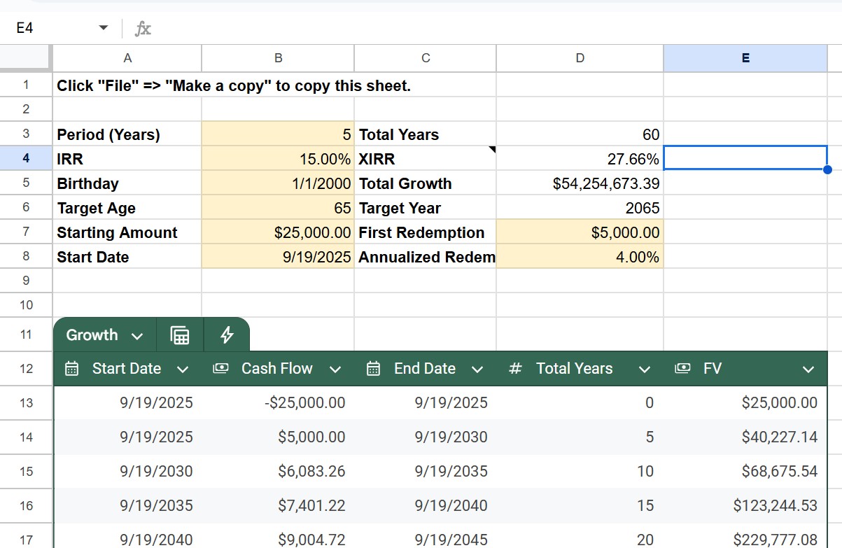
Lately, I have been working on a calculator to model the potential growth of monies in a fund that has irregular cash flows. Essentially, I am modeling what a fund that targets a specific Internal Investment Return (IRR) will deliver in growth as someone invests or redeems cash at irregular intervals.
For simplicity’s sake, the spreadsheet is designed with cash flows around a formula. This helps with achieving long-term planning, but any of the cash flows can be replaced with your own formulas or static values if there is no formulaic plan.
If you imagine any kind of tradable security as a fund, then anything can be modeled over time, assuming that an IRR has been formalized in advance. This kind of calculator is especially helpful with mutual funds and PE funds that already provide you with target IRRs though.
How does it work?
Set your period, in years; set the IRR; and set your birthday and target age. You’ll also need to set the initial investment amount and how much you plan your first redemption to be along with whatever you plan your redemption increases to be over time.
From here, the calculator’s table should fill with values. If the table isn’t long enough, just increase its length. Any table rows that have a nicely tinted green background are rows that are within your target maturity zone.

 Download the extension for
Firefox